Removing the artifacts in the spectrum

To follow this post, remember than in the first post we build a matrix with the raw NIR spectra, and that matrix is the one we are going to treat in this post to remove the spectra so we will give to the new matrix (without the artifacts). This will be the first of several conversions of the spsectra matris where we continue applying other math treatments.

First we load the libraries we are going to use and the data we prepared in the previous post:

library(tidyverse)
library(prospectr)
load("C:/BLOG/Workspaces/NIR Soil Tutorial/post2.RData")

The function we are going to use is spliceCorrection from the prospectr package. This function is used to correct the spectra for artifacts due to detector changes or other reasons. The function takes as input a matrix of spectra and returns a corrected matrix of spectra. To find information:

?prospectr::spliceCorrection

dat$spc <- spliceCorrection(dat$spc_raw, my_wavelengths, splice = c(1000, 1830))

And now we create a long version of the dataframe to plot it with ggplot2, as we have done in the second post:

spc_long <- data.frame(
sample = rep(1:nrow(dat), each = ncol(dat$spc)),
oc = rep(dat$Organic_Carbon, each = ncol(dat$spc)),
clay = rep(dat$Clay, each = ncol(dat$spc)),
silt = rep(dat$Silt, each = ncol(dat$spc)),
sand = rep(dat$Sand, each = ncol(dat$spc)),
wavelength = rep(my_wavelengths, nrow(dat)),
absorbance = as.vector(t(log(1 / dat$spc, 10))))


ggplot(
spc_long,
aes(x = wavelength, y = absorbance, group = sample, color = oc)) +
geom_line(alpha = 0.5) + # Set alpha to 0.5 for transparency
scale_color_gradient(low = 'blue', high = 'red') +
theme_minimal() +
labs(
x = 'Wavelength (nm)',
y = 'Reflectance',
color = 'Organic Carbon (%)') +
theme(legend.position = 'top')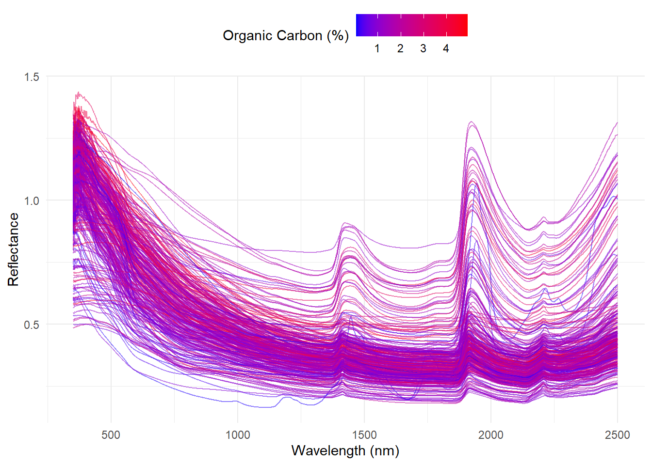

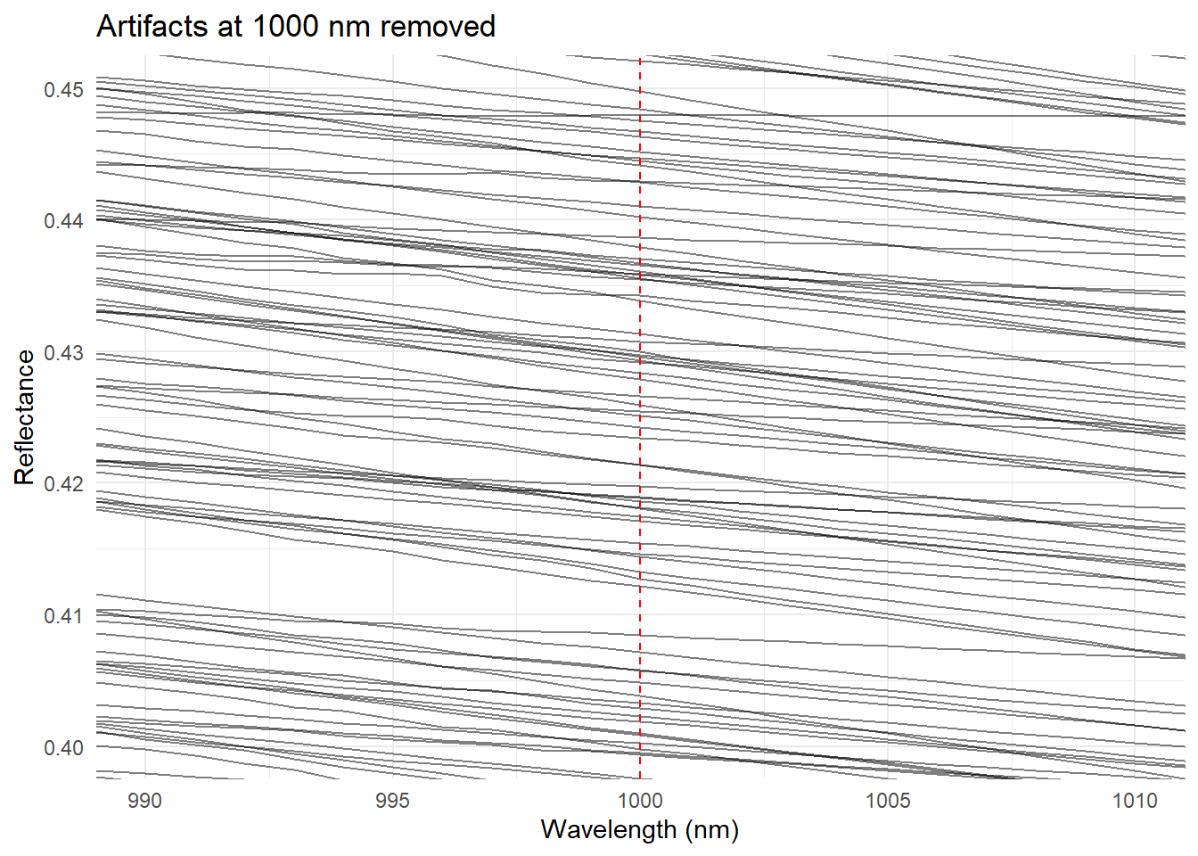
Now we can check if the artifacts are removed:

ggplot(spc_long,
       aes(x = wavelength, y = absorbance, group = sample)) +
  geom_line(alpha = 0.5) +
  theme_minimal() +
  labs(
    title = "Artifacts at 1000 nm removed",
    x = 'Wavelength (nm)',
    y = 'Reflectance'
  ) +
  coord_cartesian(xlim = c(990, 1010), ylim = c(0.4, 0.45)) +
  geom_vline(xintercept = 1000, linetype = "dashed", color = "red")